Read Data from the Cloud
Altay Sansal
Feb 12, 2026
9 min read
In this tutorial, we will use a public SEG-Y file located in Amazon Web Services’ (AWS) Simple Storage Service (S3), also known as a cloud object store.
This dataset, the Parihaka 3D full angle stack (4.7 GB per volume including full angle and near, mid, and far stacks), is provided by New Zealand Petroleum and Minerals (NZPM). Available information and data acquisition details are accessible via the SEG Wiki, the New Zealand GNS website, and the NZPM data portal.
Important
For plotting, the notebook requires Matplotlib as a dependency.
Please install it before executing using pip install matplotlib or conda install matplotlib.
Let’s start by importing some modules we will be using.
import matplotlib.pyplot as plt
from numpy.random import default_rng

from segy import SegyFile
from segy.config import SegyFileSettings
from segy.schema import HeaderField
from segy.standards import get_segy_standard
You can (but don’t) download the SEG-Y directly clicking the HTTP link from the website.
This link is convenient as the segy library supports HTTP and we can directly use it
without downloading as well. Hovewer, For demonstration purposes, we’ll use the
corresponding S3 link (or called bucket and prefix):
s3://open.source.geoscience/open_data/newzealand/Taranaiki_Basin/PARIHAKA-3D/Parihaka_PSTM_full_angle.sgy
It’s important to note that the file isn’t downloaded but rather read on demand from the
S3 object store with the segy library.
The SegyFile class uses information from the binary file header to construct a SEG-Y
spec, allowing it to read the file. The SEG-Y Revision is inferred from the binary
header by default, but can be manually set by providing a custom spec or adjusting settings.
Since this is a public bucket and an object, we need to tell S3 that we want anonymous
access, which is done by configuring storage_options in settings.
path = "s3://open.source.geoscience/open_data/newzealand/Taranaiki_Basin/PARIHAKA-3D/Parihaka_PSTM_full_angle.sgy"

# Alternatively via HTTP
# path = "http://s3.amazonaws.com/open.source.geoscience/open_data/newzealand/Taranaiki_Basin/PARIHAKA-3D/Parihaka_PSTM_full_angle.sgy"

settings = SegyFileSettings(storage_options={"anon": True})

sgy = SegyFile(path, settings=settings)
Let’s investigate the JSON version of the SEG-Y spec for this file.
Some things to note:
The opening processed inferred Revision 1 from the binary header automatically.
It generated the spec using default SEG-Y Revision 1 headers.
We can check that some headers can be defined in the wrong byte locations.
There are too many headers to deal with in the default schema.
Note that we can build this JSON independently, load it into the spec and open any SEG-Y with a schema.
sgy.spec
SegySpec(segy_standard=<SegyStandard.REV1: 1.0>, text_header=TextHeaderSpec(rows=40, cols=80, encoding=<TextHeaderEncoding.EBCDIC: 'ebcdic'>, offset=0), binary_header=HeaderSpec(fields=[HeaderField(name='job_id', byte=1, format=ScalarType.INT32), HeaderField(name='line_num', byte=5, format=ScalarType.INT32), HeaderField(name='reel_num', byte=9, format=ScalarType.INT32), HeaderField(name='data_traces_per_ensemble', byte=13, format=ScalarType.INT16), HeaderField(name='aux_traces_per_ensemble', byte=15, format=ScalarType.INT16), HeaderField(name='sample_interval', byte=17, format=ScalarType.INT16), HeaderField(name='orig_sample_interval', byte=19, format=ScalarType.INT16), HeaderField(name='samples_per_trace', byte=21, format=ScalarType.INT16), HeaderField(name='orig_samples_per_trace', byte=23, format=ScalarType.INT16), HeaderField(name='data_sample_format', byte=25, format=ScalarType.INT16), HeaderField(name='ensemble_fold', byte=27, format=ScalarType.INT16), HeaderField(name='trace_sorting_code', byte=29, format=ScalarType.INT16), HeaderField(name='vertical_sum_code', byte=31, format=ScalarType.INT16), HeaderField(name='sweep_freq_start', byte=33, format=ScalarType.INT16), HeaderField(name='sweep_freq_end', byte=35, format=ScalarType.INT16), HeaderField(name='sweep_length', byte=37, format=ScalarType.INT16), HeaderField(name='sweep_type_code', byte=39, format=ScalarType.INT16), HeaderField(name='sweep_trace_num', byte=41, format=ScalarType.INT16), HeaderField(name='sweep_taper_start', byte=43, format=ScalarType.INT16), HeaderField(name='sweep_taper_end', byte=45, format=ScalarType.INT16), HeaderField(name='taper_type_code', byte=47, format=ScalarType.INT16), HeaderField(name='correlated_data_code', byte=49, format=ScalarType.INT16), HeaderField(name='binary_gain_code', byte=51, format=ScalarType.INT16), HeaderField(name='amp_recovery_code', byte=53, format=ScalarType.INT16), HeaderField(name='measurement_system_code', byte=55, format=ScalarType.INT16), HeaderField(name='impulse_polarity_code', byte=57, format=ScalarType.INT16), HeaderField(name='vibratory_polarity_code', byte=59, format=ScalarType.INT16), HeaderField(name='segy_revision', byte=301, format=ScalarType.INT16), HeaderField(name='fixed_length_trace_flag', byte=303, format=ScalarType.INT16), HeaderField(name='num_extended_text_headers', byte=305, format=ScalarType.INT16)], item_size=400, offset=3200, endianness=<Endianness.BIG: 'big'>), ext_text_header=ExtendedTextHeaderSpec(spec=TextHeaderSpec(rows=40, cols=80, encoding=<TextHeaderEncoding.EBCDIC: 'ebcdic'>, offset=0), count=0, offset=3600), trace=TraceSpec(header=HeaderSpec(fields=[HeaderField(name='trace_seq_num_line', byte=1, format=ScalarType.INT32), HeaderField(name='trace_seq_num_reel', byte=5, format=ScalarType.INT32), HeaderField(name='orig_field_record_num', byte=9, format=ScalarType.INT32), HeaderField(name='trace_num_orig_record', byte=13, format=ScalarType.INT32), HeaderField(name='energy_source_point_num', byte=17, format=ScalarType.INT32), HeaderField(name='ensemble_num', byte=21, format=ScalarType.INT32), HeaderField(name='trace_num_ensemble', byte=25, format=ScalarType.INT32), HeaderField(name='trace_id_code', byte=29, format=ScalarType.INT16), HeaderField(name='vertically_summed_traces', byte=31, format=ScalarType.INT16), HeaderField(name='horizontally_stacked_traces', byte=33, format=ScalarType.INT16), HeaderField(name='data_use', byte=35, format=ScalarType.INT16), HeaderField(name='source_to_receiver_distance', byte=37, format=ScalarType.INT32), HeaderField(name='receiver_group_elevation', byte=41, format=ScalarType.INT32), HeaderField(name='source_surface_elevation', byte=45, format=ScalarType.INT32), HeaderField(name='source_depth_below_surface', byte=49, format=ScalarType.INT32), HeaderField(name='receiver_datum_elevation', byte=53, format=ScalarType.INT32), HeaderField(name='source_datum_elevation', byte=57, format=ScalarType.INT32), HeaderField(name='source_water_depth', byte=61, format=ScalarType.INT32), HeaderField(name='receiver_water_depth', byte=65, format=ScalarType.INT32), HeaderField(name='elevation_depth_scalar', byte=69, format=ScalarType.INT16), HeaderField(name='coordinate_scalar', byte=71, format=ScalarType.INT16), HeaderField(name='source_coord_x', byte=73, format=ScalarType.INT32), HeaderField(name='source_coord_y', byte=77, format=ScalarType.INT32), HeaderField(name='group_coord_x', byte=81, format=ScalarType.INT32), HeaderField(name='group_coord_y', byte=85, format=ScalarType.INT32), HeaderField(name='coordinate_unit', byte=89, format=ScalarType.INT16), HeaderField(name='weathering_velocity', byte=91, format=ScalarType.INT16), HeaderField(name='subweathering_velocity', byte=93, format=ScalarType.INT16), HeaderField(name='source_uphole_time', byte=95, format=ScalarType.INT16), HeaderField(name='group_uphole_time', byte=97, format=ScalarType.INT16), HeaderField(name='source_static_correction', byte=99, format=ScalarType.INT16), HeaderField(name='receiver_static_correction', byte=101, format=ScalarType.INT16), HeaderField(name='total_static_applied', byte=103, format=ScalarType.INT16), HeaderField(name='lag_time_a', byte=105, format=ScalarType.INT16), HeaderField(name='lag_time_b', byte=107, format=ScalarType.INT16), HeaderField(name='delay_recording_time', byte=109, format=ScalarType.INT16), HeaderField(name='mute_time_start', byte=111, format=ScalarType.INT16), HeaderField(name='mute_time_end', byte=113, format=ScalarType.INT16), HeaderField(name='samples_per_trace', byte=115, format=ScalarType.INT16), HeaderField(name='sample_interval', byte=117, format=ScalarType.INT16), HeaderField(name='instrument_gain_type', byte=119, format=ScalarType.INT16), HeaderField(name='instrument_gain_const', byte=121, format=ScalarType.INT16), HeaderField(name='instrument_gain_initial', byte=123, format=ScalarType.INT16), HeaderField(name='correlated_data', byte=125, format=ScalarType.INT16), HeaderField(name='sweep_freq_start', byte=127, format=ScalarType.INT16), HeaderField(name='sweep_freq_end', byte=129, format=ScalarType.INT16), HeaderField(name='sweep_length', byte=131, format=ScalarType.INT16), HeaderField(name='sweep_type', byte=133, format=ScalarType.INT16), HeaderField(name='sweep_taper_start', byte=135, format=ScalarType.INT16), HeaderField(name='sweep_taper_end', byte=137, format=ScalarType.INT16), HeaderField(name='taper_type', byte=139, format=ScalarType.INT16), HeaderField(name='alias_filter_freq', byte=141, format=ScalarType.INT16), HeaderField(name='alias_filter_slope', byte=143, format=ScalarType.INT16), HeaderField(name='notch_filter_freq', byte=145, format=ScalarType.INT16), HeaderField(name='notch_filter_slope', byte=147, format=ScalarType.INT16), HeaderField(name='low_cut_freq', byte=149, format=ScalarType.INT16), HeaderField(name='high_cut_freq', byte=151, format=ScalarType.INT16), HeaderField(name='low_cut_slope', byte=153, format=ScalarType.INT16), HeaderField(name='high_cut_slope', byte=155, format=ScalarType.INT16), HeaderField(name='year_recorded', byte=157, format=ScalarType.INT16), HeaderField(name='day_of_year', byte=159, format=ScalarType.INT16), HeaderField(name='hour_of_day', byte=161, format=ScalarType.INT16), HeaderField(name='minute_of_hour', byte=163, format=ScalarType.INT16), HeaderField(name='second_of_minute', byte=165, format=ScalarType.INT16), HeaderField(name='time_basis_code', byte=167, format=ScalarType.INT16), HeaderField(name='trace_weighting_factor', byte=169, format=ScalarType.INT16), HeaderField(name='group_num_roll_switch', byte=171, format=ScalarType.INT16), HeaderField(name='group_num_first_trace', byte=173, format=ScalarType.INT16), HeaderField(name='group_num_last_trace', byte=175, format=ScalarType.INT16), HeaderField(name='gap_size', byte=177, format=ScalarType.INT16), HeaderField(name='taper_overtravel', byte=179, format=ScalarType.INT16), HeaderField(name='cdp_x', byte=181, format=ScalarType.INT32), HeaderField(name='cdp_y', byte=185, format=ScalarType.INT32), HeaderField(name='inline', byte=189, format=ScalarType.INT32), HeaderField(name='crossline', byte=193, format=ScalarType.INT32), HeaderField(name='shot_point', byte=197, format=ScalarType.INT32), HeaderField(name='shot_point_scalar', byte=201, format=ScalarType.INT16), HeaderField(name='trace_value_unit', byte=203, format=ScalarType.INT16), HeaderField(name='transduction_const_mantissa', byte=205, format=ScalarType.INT32), HeaderField(name='transduction_const_exponent', byte=209, format=ScalarType.INT16), HeaderField(name='transduction_unit', byte=211, format=ScalarType.INT16), HeaderField(name='device_trace_id', byte=213, format=ScalarType.INT16), HeaderField(name='times_scalar', byte=215, format=ScalarType.INT16), HeaderField(name='source_type_orientation', byte=217, format=ScalarType.INT16), HeaderField(name='source_energy_dir_mantissa', byte=219, format=ScalarType.INT32), HeaderField(name='source_energy_dir_exponent', byte=223, format=ScalarType.INT16), HeaderField(name='source_measurement_mantissa', byte=225, format=ScalarType.INT32), HeaderField(name='source_measurement_exponent', byte=229, format=ScalarType.INT16), HeaderField(name='source_measurement_unit', byte=231, format=ScalarType.INT16)], item_size=240, offset=None, endianness=<Endianness.BIG: 'big'>), ext_header=None, data=TraceDataSpec(format=ScalarType.IBM32, samples=1168, interval=3000), offset=3600, endianness=<Endianness.BIG: 'big'>, count=1038162), endianness=<Endianness.BIG: 'big'>)
Let’s check the file size, number of traces, sample rate, etc. As expected, the file size matches what was in the description. We also observe there are ~ 1 million traces.
print(f"file size: {sgy.file_size / 1024**3:0.2f} GiB")
print(f"num traces: {sgy.num_traces:,}")
print(f"sample rate: {sgy.sample_interval}")
print(f"num samples: {sgy.samples_per_trace}")
print(f"sample labels: {sgy.sample_labels // 1000}")  # microsecond to millisecond
file size: 4.75 GiB
num traces: 1,038,162
sample rate: 3000
num samples: 1168
sample labels: [   0    3    6 ... 3495 3498 3501]
Using the SegyFile we can read SEG-Y components.
Here we read:
Textual file header
Binary file header
1,000 traces (headers + data) from somewhere in the middle of the file
text_header = sgy.text_header
binary_header = sgy.binary_header

start = 500_000
stop = start + 1_000

traces = sgy.trace[start:stop]

trace_headers = traces.header
trace_data = traces.sample
This should take around one second or less, based on internet connection.
Let’s print the textual header. There are a not many headers of interest. The available headers appear to be in the Revision 1 byte locations.
print(text_header)
C 1 3D VOLUME
C 2 HEADER BYTE LOCATIONS AND TYPES:
C 3     3D INLINE : 189-192 (4-BYTE INT)    3D CROSSLINE: 193-196 (4-BYTE INT)
C 4     ENSEMBLE X: 181-184 (4-BYTE INT)    ENSEMBLE Y  : 185-188 (4-BYTE INT)
C 5
C 6 SAMPLES/TRACE     :       1168
C 7 SAMPLE INTERVAL   :       3000 microseconds
C 8 FIRST SAMPLE AT   :          0 ms
C 9 VERTICAL DIMENSION: TWT (ms)
C10 SAMPLE RECORDING FORMAT: IBM FLOATING POINT (4-BYTE)
C11
C12
C13
C14
C15
C16
C17
C18
C19
C20
C21
C22
C23
C24
C25
C26
C27
C28
C29
C30
C31
C32
C33
C34
C35
C36
C37
C38 WRITTEN BY INSIGHT VERSION 3.0 (405040)               http://www.dugsw.com/
C39 SEG Y REV1
C40 END TEXTUAL HEADER
We can look at headers (by default it is a Pandas DataFrame) in a nicely formatted table.
We can also do typical Pandas analytics (like plots, statistics, etc.) but it won’t be shown here.
binary_header.to_dataframe()
| job_id | line_num | reel_num | data_traces_per_ensemble | aux_traces_per_ensemble | sample_interval | orig_sample_interval | samples_per_trace | orig_samples_per_trace | data_sample_format | ... | correlated_data_code | binary_gain_code | amp_recovery_code | measurement_system_code | impulse_polarity_code | vibratory_polarity_code | fixed_length_trace_flag | num_extended_text_headers | segy_revision_major | segy_revision_minor | |
|---|---|---|---|---|---|---|---|---|---|---|---|---|---|---|---|---|---|---|---|---|---|
| 0 | 0 | 0 | 0 | 0 | 0 | 3000 | 0 | 1168 | 0 | 1 | ... | 0 | 0 | 0 | 0 | 0 | 0 | 1 | 0 | 1 | 0 |
1 rows × 31 columns
trace_headers.to_dataframe()
| trace_seq_num_line | trace_seq_num_reel | orig_field_record_num | trace_num_orig_record | energy_source_point_num | ensemble_num | trace_num_ensemble | trace_id_code | vertically_summed_traces | horizontally_stacked_traces | ... | transduction_const_exponent | transduction_unit | device_trace_id | times_scalar | source_type_orientation | source_energy_dir_mantissa | source_energy_dir_exponent | source_measurement_mantissa | source_measurement_exponent | source_measurement_unit | |
|---|---|---|---|---|---|---|---|---|---|---|---|---|---|---|---|---|---|---|---|---|---|
| 0 | 0 | 0 | 0 | 0 | 0 | 0 | 0 | 0 | 0 | 0 | ... | 0 | 0 | 0 | 0 | 0 | 0 | 0 | 0 | 0 | 0 |
| 1 | 0 | 0 | 0 | 0 | 0 | 0 | 0 | 0 | 0 | 0 | ... | 0 | 0 | 0 | 0 | 0 | 0 | 0 | 0 | 0 | 0 |
| 2 | 0 | 0 | 0 | 0 | 0 | 0 | 0 | 0 | 0 | 0 | ... | 0 | 0 | 0 | 0 | 0 | 0 | 0 | 0 | 0 | 0 |
| 3 | 0 | 0 | 0 | 0 | 0 | 0 | 0 | 0 | 0 | 0 | ... | 0 | 0 | 0 | 0 | 0 | 0 | 0 | 0 | 0 | 0 |
| 4 | 0 | 0 | 0 | 0 | 0 | 0 | 0 | 0 | 0 | 0 | ... | 0 | 0 | 0 | 0 | 0 | 0 | 0 | 0 | 0 | 0 |
| ... | ... | ... | ... | ... | ... | ... | ... | ... | ... | ... | ... | ... | ... | ... | ... | ... | ... | ... | ... | ... | ... |
| 995 | 0 | 0 | 0 | 0 | 0 | 0 | 0 | 0 | 0 | 0 | ... | 0 | 0 | 0 | 0 | 0 | 0 | 0 | 0 | 0 | 0 |
| 996 | 0 | 0 | 0 | 0 | 0 | 0 | 0 | 0 | 0 | 0 | ... | 0 | 0 | 0 | 0 | 0 | 0 | 0 | 0 | 0 | 0 |
| 997 | 0 | 0 | 0 | 0 | 0 | 0 | 0 | 0 | 0 | 0 | ... | 0 | 0 | 0 | 0 | 0 | 0 | 0 | 0 | 0 | 0 |
| 998 | 0 | 0 | 0 | 0 | 0 | 0 | 0 | 0 | 0 | 0 | ... | 0 | 0 | 0 | 0 | 0 | 0 | 0 | 0 | 0 | 0 |
| 999 | 0 | 0 | 0 | 0 | 0 | 0 | 0 | 0 | 0 | 0 | ... | 0 | 0 | 0 | 0 | 0 | 0 | 0 | 0 | 0 | 0 |
1000 rows × 89 columns
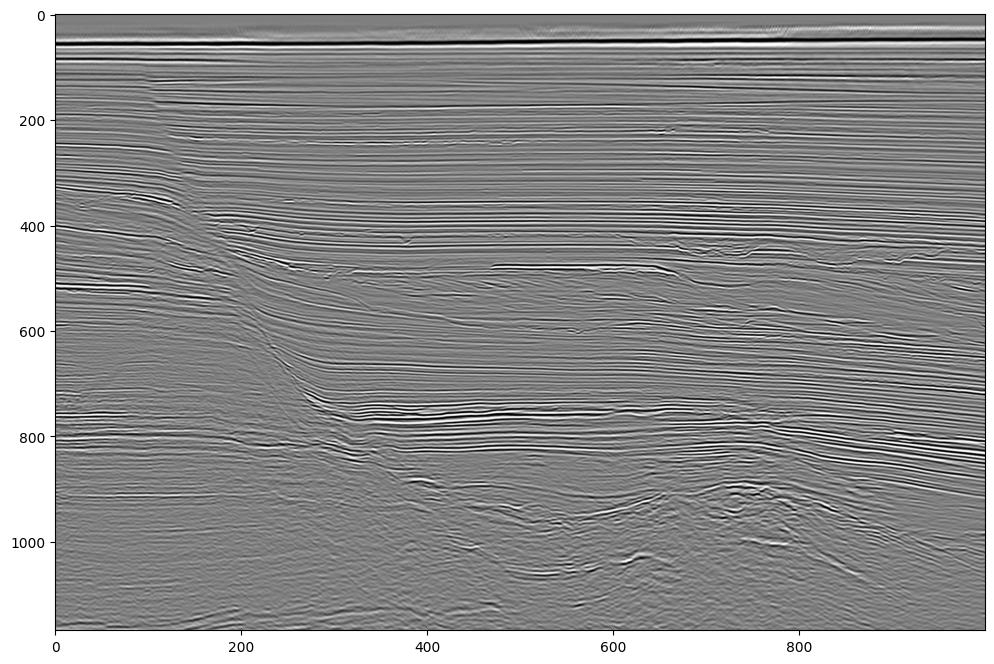
Let’s plot the traces.
Note that they are all parsed from IBM floats to IEEE floats (decoded) in the background.
plt.figure(figsize=(12, 8))
plot_kw = {"aspect": "auto", "cmap": "gray_r", "interpolation": "bilinear"}
plt.imshow(trace_data.T, vmin=-1000, vmax=1000, **plot_kw);
With Custom Spec
We will create a new custom spec based on SEG-Y revision 1 with different binary and trace header fields. This way, we will parse ONLY the parts we want, with correct byte locations.
A user can define a completely custom SEG-Y spec from scratch as well, but for convenience, we are customizing the Revision 1 schema with the parts that we want to change.
Note that doing this will also modify the segyStandard field to None to
ensure we don’t assume the file schema is standard after doing this.
From the binary file header, we will read:
Number of samples
Sample rate
From the trace headers, we will read:
Inline
Crossline
CDP-X
CDP-Y
Coordinate scalar
Based on the text header lines:
C 2 HEADER BYTE LOCATIONS AND TYPES:
C 3     3D INLINE : 189-192 (4-BYTE INT)    3D CROSSLINE: 193-196 (4-BYTE INT)
C 4     ENSEMBLE X: 181-184 (4-BYTE INT)    ENSEMBLE Y  : 185-188 (4-BYTE INT)
As we know by the SEG-Y Rev1 definition, the coordinate scalars are at byte 71.
rev1 = get_segy_standard(1.0)
custom_spec = rev1.customize(
    binary_header_fields=[
        HeaderField(name="sample_interval", byte=17, format="int16"),
        HeaderField(name="samples_per_trace", byte=21, format="int16"),
        HeaderField(name="data_sample_format", byte=25, format="int16"),
        HeaderField(name="num_extended_text_headers", byte=305, format="int16"),
    ],
    trace_header_fields=[
        HeaderField(name="inline", byte=189, format="int32"),
        HeaderField(name="crossline", byte=193, format="int32"),
        HeaderField(name="cdp_x", byte=181, format="int32"),
        HeaderField(name="cdp_y", byte=185, format="int32"),
        HeaderField(name="coordinate_scalar", byte=71, format="int16"),
    ],
)

sgy = SegyFile(path, spec=custom_spec, settings=settings)
Now let’s look at the spec again. It is a lot more compact.
sgy.spec
SegySpec(segy_standard=<SegyStandard.REV1: 1.0>, text_header=TextHeaderSpec(rows=40, cols=80, encoding=<TextHeaderEncoding.EBCDIC: 'ebcdic'>, offset=0), binary_header=HeaderSpec(fields=[HeaderField(name='job_id', byte=1, format=ScalarType.INT32), HeaderField(name='line_num', byte=5, format=ScalarType.INT32), HeaderField(name='reel_num', byte=9, format=ScalarType.INT32), HeaderField(name='data_traces_per_ensemble', byte=13, format=ScalarType.INT16), HeaderField(name='aux_traces_per_ensemble', byte=15, format=ScalarType.INT16), HeaderField(name='sample_interval', byte=17, format=ScalarType.INT16), HeaderField(name='orig_sample_interval', byte=19, format=ScalarType.INT16), HeaderField(name='samples_per_trace', byte=21, format=ScalarType.INT16), HeaderField(name='orig_samples_per_trace', byte=23, format=ScalarType.INT16), HeaderField(name='data_sample_format', byte=25, format=ScalarType.INT16), HeaderField(name='ensemble_fold', byte=27, format=ScalarType.INT16), HeaderField(name='trace_sorting_code', byte=29, format=ScalarType.INT16), HeaderField(name='vertical_sum_code', byte=31, format=ScalarType.INT16), HeaderField(name='sweep_freq_start', byte=33, format=ScalarType.INT16), HeaderField(name='sweep_freq_end', byte=35, format=ScalarType.INT16), HeaderField(name='sweep_length', byte=37, format=ScalarType.INT16), HeaderField(name='sweep_type_code', byte=39, format=ScalarType.INT16), HeaderField(name='sweep_trace_num', byte=41, format=ScalarType.INT16), HeaderField(name='sweep_taper_start', byte=43, format=ScalarType.INT16), HeaderField(name='sweep_taper_end', byte=45, format=ScalarType.INT16), HeaderField(name='taper_type_code', byte=47, format=ScalarType.INT16), HeaderField(name='correlated_data_code', byte=49, format=ScalarType.INT16), HeaderField(name='binary_gain_code', byte=51, format=ScalarType.INT16), HeaderField(name='amp_recovery_code', byte=53, format=ScalarType.INT16), HeaderField(name='measurement_system_code', byte=55, format=ScalarType.INT16), HeaderField(name='impulse_polarity_code', byte=57, format=ScalarType.INT16), HeaderField(name='vibratory_polarity_code', byte=59, format=ScalarType.INT16), HeaderField(name='segy_revision', byte=301, format=ScalarType.INT16), HeaderField(name='fixed_length_trace_flag', byte=303, format=ScalarType.INT16), HeaderField(name='num_extended_text_headers', byte=305, format=ScalarType.INT16)], item_size=400, offset=3200, endianness=<Endianness.BIG: 'big'>), ext_text_header=ExtendedTextHeaderSpec(spec=TextHeaderSpec(rows=40, cols=80, encoding=<TextHeaderEncoding.EBCDIC: 'ebcdic'>, offset=0), count=0, offset=3600), trace=TraceSpec(header=HeaderSpec(fields=[HeaderField(name='trace_seq_num_line', byte=1, format=ScalarType.INT32), HeaderField(name='trace_seq_num_reel', byte=5, format=ScalarType.INT32), HeaderField(name='orig_field_record_num', byte=9, format=ScalarType.INT32), HeaderField(name='trace_num_orig_record', byte=13, format=ScalarType.INT32), HeaderField(name='energy_source_point_num', byte=17, format=ScalarType.INT32), HeaderField(name='ensemble_num', byte=21, format=ScalarType.INT32), HeaderField(name='trace_num_ensemble', byte=25, format=ScalarType.INT32), HeaderField(name='trace_id_code', byte=29, format=ScalarType.INT16), HeaderField(name='vertically_summed_traces', byte=31, format=ScalarType.INT16), HeaderField(name='horizontally_stacked_traces', byte=33, format=ScalarType.INT16), HeaderField(name='data_use', byte=35, format=ScalarType.INT16), HeaderField(name='source_to_receiver_distance', byte=37, format=ScalarType.INT32), HeaderField(name='receiver_group_elevation', byte=41, format=ScalarType.INT32), HeaderField(name='source_surface_elevation', byte=45, format=ScalarType.INT32), HeaderField(name='source_depth_below_surface', byte=49, format=ScalarType.INT32), HeaderField(name='receiver_datum_elevation', byte=53, format=ScalarType.INT32), HeaderField(name='source_datum_elevation', byte=57, format=ScalarType.INT32), HeaderField(name='source_water_depth', byte=61, format=ScalarType.INT32), HeaderField(name='receiver_water_depth', byte=65, format=ScalarType.INT32), HeaderField(name='elevation_depth_scalar', byte=69, format=ScalarType.INT16), HeaderField(name='coordinate_scalar', byte=71, format=ScalarType.INT16), HeaderField(name='source_coord_x', byte=73, format=ScalarType.INT32), HeaderField(name='source_coord_y', byte=77, format=ScalarType.INT32), HeaderField(name='group_coord_x', byte=81, format=ScalarType.INT32), HeaderField(name='group_coord_y', byte=85, format=ScalarType.INT32), HeaderField(name='coordinate_unit', byte=89, format=ScalarType.INT16), HeaderField(name='weathering_velocity', byte=91, format=ScalarType.INT16), HeaderField(name='subweathering_velocity', byte=93, format=ScalarType.INT16), HeaderField(name='source_uphole_time', byte=95, format=ScalarType.INT16), HeaderField(name='group_uphole_time', byte=97, format=ScalarType.INT16), HeaderField(name='source_static_correction', byte=99, format=ScalarType.INT16), HeaderField(name='receiver_static_correction', byte=101, format=ScalarType.INT16), HeaderField(name='total_static_applied', byte=103, format=ScalarType.INT16), HeaderField(name='lag_time_a', byte=105, format=ScalarType.INT16), HeaderField(name='lag_time_b', byte=107, format=ScalarType.INT16), HeaderField(name='delay_recording_time', byte=109, format=ScalarType.INT16), HeaderField(name='mute_time_start', byte=111, format=ScalarType.INT16), HeaderField(name='mute_time_end', byte=113, format=ScalarType.INT16), HeaderField(name='samples_per_trace', byte=115, format=ScalarType.INT16), HeaderField(name='sample_interval', byte=117, format=ScalarType.INT16), HeaderField(name='instrument_gain_type', byte=119, format=ScalarType.INT16), HeaderField(name='instrument_gain_const', byte=121, format=ScalarType.INT16), HeaderField(name='instrument_gain_initial', byte=123, format=ScalarType.INT16), HeaderField(name='correlated_data', byte=125, format=ScalarType.INT16), HeaderField(name='sweep_freq_start', byte=127, format=ScalarType.INT16), HeaderField(name='sweep_freq_end', byte=129, format=ScalarType.INT16), HeaderField(name='sweep_length', byte=131, format=ScalarType.INT16), HeaderField(name='sweep_type', byte=133, format=ScalarType.INT16), HeaderField(name='sweep_taper_start', byte=135, format=ScalarType.INT16), HeaderField(name='sweep_taper_end', byte=137, format=ScalarType.INT16), HeaderField(name='taper_type', byte=139, format=ScalarType.INT16), HeaderField(name='alias_filter_freq', byte=141, format=ScalarType.INT16), HeaderField(name='alias_filter_slope', byte=143, format=ScalarType.INT16), HeaderField(name='notch_filter_freq', byte=145, format=ScalarType.INT16), HeaderField(name='notch_filter_slope', byte=147, format=ScalarType.INT16), HeaderField(name='low_cut_freq', byte=149, format=ScalarType.INT16), HeaderField(name='high_cut_freq', byte=151, format=ScalarType.INT16), HeaderField(name='low_cut_slope', byte=153, format=ScalarType.INT16), HeaderField(name='high_cut_slope', byte=155, format=ScalarType.INT16), HeaderField(name='year_recorded', byte=157, format=ScalarType.INT16), HeaderField(name='day_of_year', byte=159, format=ScalarType.INT16), HeaderField(name='hour_of_day', byte=161, format=ScalarType.INT16), HeaderField(name='minute_of_hour', byte=163, format=ScalarType.INT16), HeaderField(name='second_of_minute', byte=165, format=ScalarType.INT16), HeaderField(name='time_basis_code', byte=167, format=ScalarType.INT16), HeaderField(name='trace_weighting_factor', byte=169, format=ScalarType.INT16), HeaderField(name='group_num_roll_switch', byte=171, format=ScalarType.INT16), HeaderField(name='group_num_first_trace', byte=173, format=ScalarType.INT16), HeaderField(name='group_num_last_trace', byte=175, format=ScalarType.INT16), HeaderField(name='gap_size', byte=177, format=ScalarType.INT16), HeaderField(name='taper_overtravel', byte=179, format=ScalarType.INT16), HeaderField(name='cdp_x', byte=181, format=ScalarType.INT32), HeaderField(name='cdp_y', byte=185, format=ScalarType.INT32), HeaderField(name='inline', byte=189, format=ScalarType.INT32), HeaderField(name='crossline', byte=193, format=ScalarType.INT32), HeaderField(name='shot_point', byte=197, format=ScalarType.INT32), HeaderField(name='shot_point_scalar', byte=201, format=ScalarType.INT16), HeaderField(name='trace_value_unit', byte=203, format=ScalarType.INT16), HeaderField(name='transduction_const_mantissa', byte=205, format=ScalarType.INT32), HeaderField(name='transduction_const_exponent', byte=209, format=ScalarType.INT16), HeaderField(name='transduction_unit', byte=211, format=ScalarType.INT16), HeaderField(name='device_trace_id', byte=213, format=ScalarType.INT16), HeaderField(name='times_scalar', byte=215, format=ScalarType.INT16), HeaderField(name='source_type_orientation', byte=217, format=ScalarType.INT16), HeaderField(name='source_energy_dir_mantissa', byte=219, format=ScalarType.INT32), HeaderField(name='source_energy_dir_exponent', byte=223, format=ScalarType.INT16), HeaderField(name='source_measurement_mantissa', byte=225, format=ScalarType.INT32), HeaderField(name='source_measurement_exponent', byte=229, format=ScalarType.INT16), HeaderField(name='source_measurement_unit', byte=231, format=ScalarType.INT16)], item_size=240, offset=None, endianness=<Endianness.BIG: 'big'>), ext_header=None, data=TraceDataSpec(format=ScalarType.IBM32, samples=1168, interval=3000), offset=3600, endianness=<Endianness.BIG: 'big'>, count=1038162), endianness=<Endianness.BIG: 'big'>)
As mentioned earlier, the JSON can be laded into the spec from a file too.
1from segy.schema import SegySpec
2import os
3
4json_path = "..."
5
6with open(json_path, mode="r") as fp:
7    data = fp.read()
8    spec = SegySpec.model_validate_json(data)
Let’s do something a little more interesting now. Let’s try to plot a time slice by randomly sampling the file.
We will read 5,000 random traces. This should take about 15-20 seconds, based on your internet connection speed.
text_header = sgy.text_header
binary_header = sgy.binary_header

rng = default_rng()
indices = rng.choice(sgy.num_traces, size=5_000, replace=False)

traces = sgy.trace[indices]
binary_header.to_dataframe()
| job_id | line_num | reel_num | data_traces_per_ensemble | aux_traces_per_ensemble | sample_interval | orig_sample_interval | samples_per_trace | orig_samples_per_trace | data_sample_format | ... | correlated_data_code | binary_gain_code | amp_recovery_code | measurement_system_code | impulse_polarity_code | vibratory_polarity_code | fixed_length_trace_flag | num_extended_text_headers | segy_revision_major | segy_revision_minor | |
|---|---|---|---|---|---|---|---|---|---|---|---|---|---|---|---|---|---|---|---|---|---|
| 0 | 0 | 0 | 0 | 0 | 0 | 3000 | 0 | 1168 | 0 | 1 | ... | 0 | 0 | 0 | 0 | 0 | 0 | 1 | 0 | 1 | 0 |
1 rows × 31 columns
trace_headers = traces.header.to_dataframe()

trace_headers["cdp_x"] /= trace_headers["coordinate_scalar"].abs()
trace_headers["cdp_y"] /= trace_headers["coordinate_scalar"].abs()

trace_headers
| trace_seq_num_line | trace_seq_num_reel | orig_field_record_num | trace_num_orig_record | energy_source_point_num | ensemble_num | trace_num_ensemble | trace_id_code | vertically_summed_traces | horizontally_stacked_traces | ... | transduction_const_exponent | transduction_unit | device_trace_id | times_scalar | source_type_orientation | source_energy_dir_mantissa | source_energy_dir_exponent | source_measurement_mantissa | source_measurement_exponent | source_measurement_unit | |
|---|---|---|---|---|---|---|---|---|---|---|---|---|---|---|---|---|---|---|---|---|---|
| 0 | 0 | 0 | 0 | 0 | 0 | 0 | 0 | 0 | 0 | 0 | ... | 0 | 0 | 0 | 0 | 0 | 0 | 0 | 0 | 0 | 0 |
| 1 | 0 | 0 | 0 | 0 | 0 | 0 | 0 | 0 | 0 | 0 | ... | 0 | 0 | 0 | 0 | 0 | 0 | 0 | 0 | 0 | 0 |
| 2 | 0 | 0 | 0 | 0 | 0 | 0 | 0 | 0 | 0 | 0 | ... | 0 | 0 | 0 | 0 | 0 | 0 | 0 | 0 | 0 | 0 |
| 3 | 0 | 0 | 0 | 0 | 0 | 0 | 0 | 0 | 0 | 0 | ... | 0 | 0 | 0 | 0 | 0 | 0 | 0 | 0 | 0 | 0 |
| 4 | 0 | 0 | 0 | 0 | 0 | 0 | 0 | 0 | 0 | 0 | ... | 0 | 0 | 0 | 0 | 0 | 0 | 0 | 0 | 0 | 0 |
| ... | ... | ... | ... | ... | ... | ... | ... | ... | ... | ... | ... | ... | ... | ... | ... | ... | ... | ... | ... | ... | ... |
| 4995 | 0 | 0 | 0 | 0 | 0 | 0 | 0 | 0 | 0 | 0 | ... | 0 | 0 | 0 | 0 | 0 | 0 | 0 | 0 | 0 | 0 |
| 4996 | 0 | 0 | 0 | 0 | 0 | 0 | 0 | 0 | 0 | 0 | ... | 0 | 0 | 0 | 0 | 0 | 0 | 0 | 0 | 0 | 0 |
| 4997 | 0 | 0 | 0 | 0 | 0 | 0 | 0 | 0 | 0 | 0 | ... | 0 | 0 | 0 | 0 | 0 | 0 | 0 | 0 | 0 | 0 |
| 4998 | 0 | 0 | 0 | 0 | 0 | 0 | 0 | 0 | 0 | 0 | ... | 0 | 0 | 0 | 0 | 0 | 0 | 0 | 0 | 0 | 0 |
| 4999 | 0 | 0 | 0 | 0 | 0 | 0 | 0 | 0 | 0 | 0 | ... | 0 | 0 | 0 | 0 | 0 | 0 | 0 | 0 | 0 | 0 |
5000 rows × 89 columns
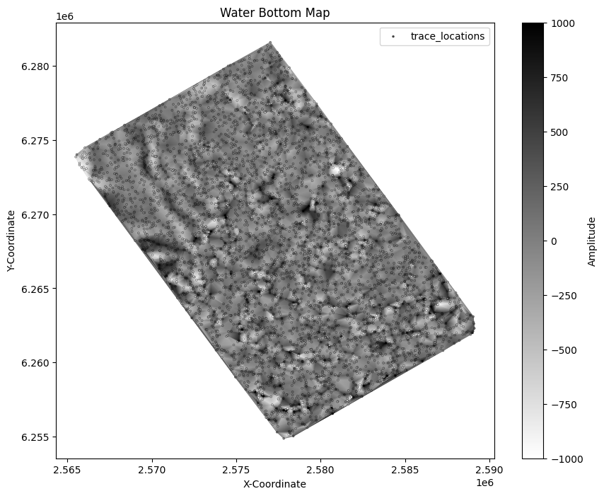
Now we can plot the time slice on actual coordinates from the headers and even see a hint of the outline of the data! Since we significantly down-sampled the data, the time slice is aliased and not very useful, but this shows us the concept of making maps.
plt.figure(figsize=(10, 8))

z_slice_index = 500

x, y, z = (
    trace_headers["cdp_x"],
    trace_headers["cdp_y"],
    traces.sample[:, z_slice_index],
)

scatter_kw = {"ec": [0.0, 0.0, 0.0, 0.5], "linewidth": 0.5}
color_kw = {"cmap": "gray_r", "vmin": -1000, "vmax": 1000}

plt.tripcolor(x, y, z, shading="gouraud", **color_kw)
plt.scatter(x, y, s=4, c=z, label="trace_locations", **scatter_kw, **color_kw)
plt.title("Water Bottom Map")
plt.colorbar(label="Amplitude")
plt.xlabel("X-Coordinate")
plt.ylabel("Y-Coordinate")
plt.legend();